Predictions on Private Equity Fund’s Contribution Using Encoder-Decoder LSTM Model with Multivariate Input

• Link to Github

• Full Report

This project is trying to model the contribution and distribution of PE funds. They are time related characters, especially when using the rate of contribution (percentage of capital commitment).

Introduction

Private Equity, a fast growing part in the past years in the financial sector, attracts investors attention as they give alternatives investment for people who would like to take illiquidity risk with higher rewards in return. PE firms mainly focus on primary markets. They invest in companies in their early stages to own a share of such company and sell it later to other investors or to the public. This business model is recognized as a very profitable one in the industry. However, from an investor’s perspective, it is hard to predict the cash flows of PE companies as well as returns for investors due to illiquid nature of assets and lack of accessible data.

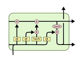
In our work, we kept the LSTM structure in our models since the memory capability of the LSTM works perfect in this situation. The cell state is saving some of the cash flows that were observed in the previous quarters, the forget layer decides which of those cash flows to forget, the middle layers train the data and pass it through the cell state (adding new data or updating previous data that was stored) and the output layer performs the double filter to obtain the predictions.

Data

The data part includes the description of the data we used, the process procedure and other experiments and exploration we did to get more data.

Data Description and Processing

We used the 5-year quarterly benchmarks data for the 3 types of funds downloaded from Preqin as source data. Based on the assumption used in many papers, we also assume that the call-up and distribution of PE funds take lognormal distribution. Therefore, instead of replicating the call-up and distribution themselves, we computed the change of the data after log transformation followed by linear interpolation and adding Gaussian noise to expand the log difference to daily data.

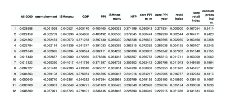
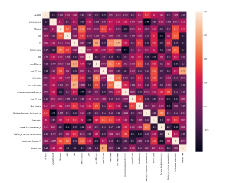
In addition, we selected 20 macro factors and got their historical data of the same time period.

Data Exploration and Databases

We mainly explored the following two databases: Preqin and Capital IQ.

Preqin is a database focusing on PE and VC funds. Under the Performance tag, we can see fund specific historical performance data. Users have access to download two kinds of performance data: historical funds info data and funds specific historical performance data.

Models Architectures and Input Variables

Our group’s objective is to improve the performance of the model by changing the model architecture, while keeping the interpolation method (stochastic interpolation), prediction horizon (360 days in the future), and length of historical data for prediction (270 days) the same. Based on the prototype model they have built, our group keep the optimizer and training epoch the same (Adam Optimizer & 100 epochs), and mainly modify the architecture to create the following models:

1. Baseline LSTM Model
2. Encoder-Decoder LSTM Model
3. CNN-LSTM Encoder-Decoder Model
4. ConvLSTM Encoder-Decoder Model

For each architectures, we test them on different types of input:

1. Univariate input with only Fund’s cash-flow data
2. Multivariate input with cash-flow data and all macroeconomic factors we found
3. Multivariate input with cash-flow data and macroeconomic factors selected by Principal Component Analysis (PCA)

Architecture

Baseline LSTM Model

For the vanilla LSTM model, we try to keep the most of the previous architecture, such as optimizer, the number of layers, epochs and loss function. However, we encounter the exploding gradient problem when we make the prediction. Though we have tried to use clip value, R2 regularization and batch normalization to put constraints on the weight, it doesn’t perform as desired. Also, as the previous mentioned that they experienced vanishing gradient problems and periodic results, for the first problem we changed the state activation function to ReLU and keep this change for the further models, for the second one we continue to use mini-batch size equal to 100 to avoid periodic prediction.

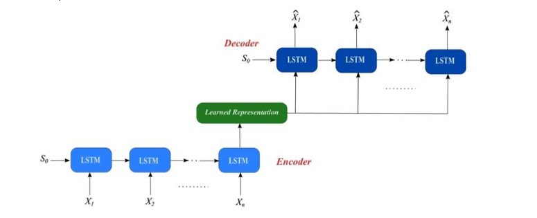
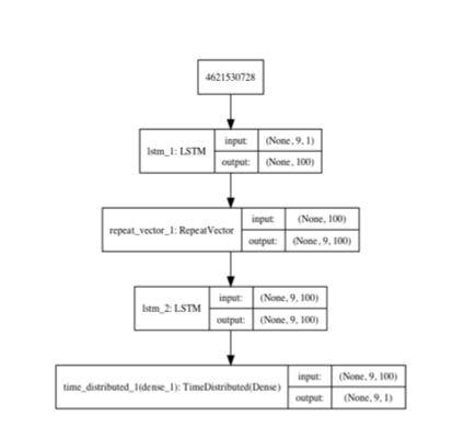
Encoder-Decoder LSTM Model

Rather than directly output the sequence to the fully connected layer, the encoder-decoder LSTM model has two sub-models, one as the encoder to take original 10 input sequence and encode it, then the decoder read the encoded output as the next LSTM input sequence. The main difference here is that the LSTM model used in the decoder will know the predicted output from the previous LSTM and use that as an input to further generate the outputs, then passing to the fully connected layers, which in this case will be a TimeDistributed wrapper functionally the same as fully connected layers with only the encoder outputs become three dimensions, and example is demonstrated below (Srivastava, Mansimov, Salakhutdinov, 2015). This structure is more often used and performs better in multivariate time series forecasting problems(Sagheer & Kotb, 2019).

CNN-LSTM Encoder-Decoder Model

While LSTM could be used as the encoder, a convolutional neural network is able to perform similarly as an encoder as well. Though it is used in computer vision in most cases(Donahue al), CNN-LSTM model can also be used for time series data forecasting, especially for multivariate inputs(Du, Li & Yang, 2018). The CNN encoder can learn the relationship between time series data horizontally, in our case is how Funds’ cash flow interacts with macroeconomic features like GDP, interest rate, etc. In this model we add two 1-d convolutional layers, and use 64 filters with kernel size equal to 3, and finally use the max pooling (2) to keep 1/4 of the values.

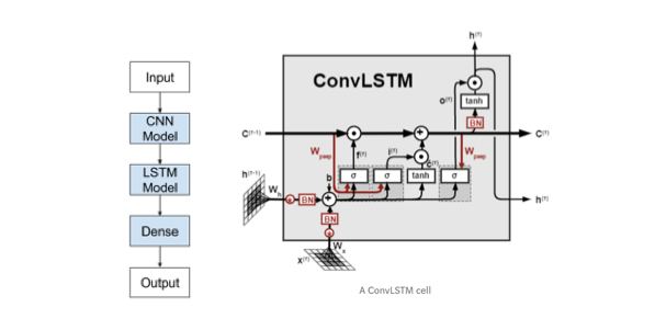
ConvLSTM Encoder-Decoder Model

On the top of CNN-LSTM model, ConvLSTM is a further extension to what we have by now, which directly uses convolutions in reading the raw data, rather than take it to encoder CNN and interpret the output (see A ConvLSTM cell above). This model has a better performance in capturing spatiotemporal correlations(Shi, Chen & Wang, 2015). In our case, the combination of funds’ cash flow macro economic factors could be interpreted as the two-dimension pixel data in the image input. Then we set the number of subsequences in ConvLSTM2D layer yo be 3 and change the length of each subsequence to 90, which makes the multiple of them equal to the original history length 270. This hyperparameter set up is intuitively straightforward as our raw data is on a quarterly basis, and we have performed stochastic interpolation between two given data values to generate 90 days data.

Variables

The primary feature we used to forecast is the interpolated log return of contribution cash flow (Called Up) for Buyout (All), Real Estate, and Venture Capital Funds. The data and interpolation method is exactly the same with the previous group so that we can make the results more comparable.

Result Comparison and Discussion

Project Result

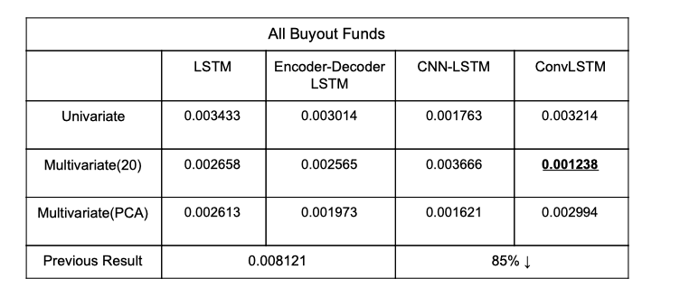
The previous team has achieved impressive Mean Square Errors under both training set and testing with 100 epochs and the sequence length of 270 for the data we used in All-Buyout, Real Estate and VC funds, which are all below 0.01. However, they experienced noisy predictions for both train and test set and the prediction curve seems to fluctuate up and down for all types of funds. Additionally, the models they built tend to overpredict the log return value in the test set by 0.05. After the changes in the architecture, our models tend to be more smooth and the overprediction problem has been eased in some of the models, especially in the Real Estate funds data - the data that achieve the best MSE performance for the previous group. It could possibly be the change in architecture, parameters and activation functions that make this improvement possible.

• Result For Buyout Funds

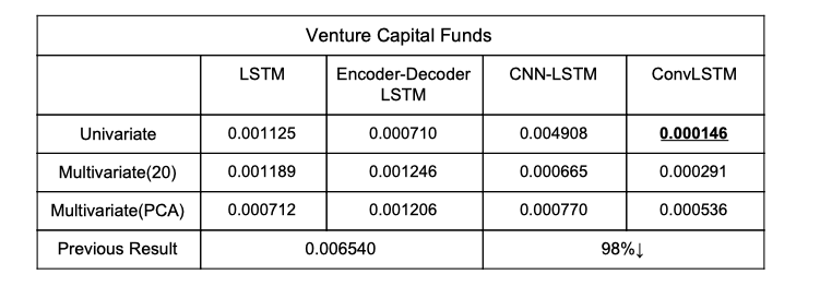
• Result For Venture Capital Funds

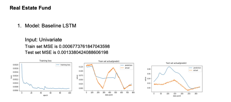
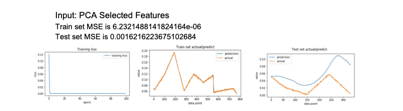
Visualization of Loss Function and Actual/Predict

• Left: Training Loss
• Mid: Training Set Actual Value/Prediction
• Right: Testing Set Actual Value/Prediction

Here are some visualization for the training and testing result, for more demonstration please refer to the full report

• Fund: Real Estate Funds
• Model: Baseline LSTM

• Input: Univariate

• Fund: Buyout Funds
• Model: CNN-LSTM
• Input: PCA

Conclusion and Future Improvements

Our main aim was to ameliorate the modeling that was done by the previous group by building on their LSTM model for one year in advanced prediction of contributions and distributions of buyout PE funds.

There are many directions which one could take to further this project. One would be to replace the classical stochastic bridge interpolation with something more robust like a variance gamma brownian bridge or even a deep Conditional Generative Adversarial Network. You could also use ensemble methods to combine different LSTM models to achieve a better less overfit model. Moreover, you could try and get more contribution distribution data for all the kinds of PE funds in order to have a larger training set for each model. We contacted the service of Preqin and were notified that the fund specific historical performance data might be obtained through special requests and fees might be applied. If this work is intended to go deeper, a sufficient and robust dataset is required. Furthermore you could also experiment with replacing the LSTM model with another time series model, such as an auto regressive one, to make a different benchmark for model performance. You could even feed the result from the autoregressive model as another feature in the LSTM model and see how that affects the performance.