NBA Shot Prediction - Maximizing Chances of Victory in Basketball

• Link to Github
• Full Report

Project Overview

Our objective is to build a shot prediction model, whether the player will score or not score, based on the data analysis that we conduct after taking the shots and the circumstances under which they are made into consideration, to help all stakeholders develop more effective game strategies. In building our models, our data mining goal is to find the best model that has the highest accuracy and F1-score.

Data Understanding & Preparation

We will first explain our original dataset before explaining how it is prepared. Afterwards, we will explore our new, blended dataset using exploratory data visualization (EDA) methods.

The dataset is a public Kaggle dataset that records all the shots attempted during the NBA 2014-2015 season. It is uploaded by a Kaggle data scientist named “DanB”, and he derived the raw data from NBA’s REST API. The target variable is the “Shot Result”, whether the player made the shot (“made”) or missed the shot (“missed”). There is a total of 128,069 data point (or shots attempted), each with 20 variables explaining the shot’s feature. The completeness of the dataset is quite high, but the depth of information on players is quite shallow. We thus decided to find another dataset on players’ personal information.

Link to the original dataset

Data Preparation Steps

We followed the 5 essential data preparation steps to create our ideal dataset. First, we gathered NBA players’ seasonal data from Kaggle1 and used Vlookup in Excel to link our original dataset’s variables “Closest Defender’s Name” and “Player” to their seasonal data. Second, we cleaned our dataset through deleting 70 variables that we deem unnecessary, such as offense variables in defenders and defend variables in offenders. We then renamed predictor variable fields so that we could conduct data blending, or matching the correct player data to the shots’ data. Lastly, we did data sampling by taking out data entries that we found to be outliers. Our finalized dataset has 127,951 observations with 46 variables.

Data Understanding Using Visualization

This session will illustrate relationship between pairs or small numbers of attributes using different visualization techniques.

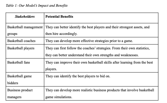
• The Box Plot

The Box Plot illustrates the relationship between the height of players and their positions in teams. Intuitively, players with center positions, who are normally the last line of defense in an offensive attempt, needs to be the tallest. Similarly, players who are point guards usually are ball-handler and requires a relatively smaller physique to agilely move around in the field.

• Distribution Plot

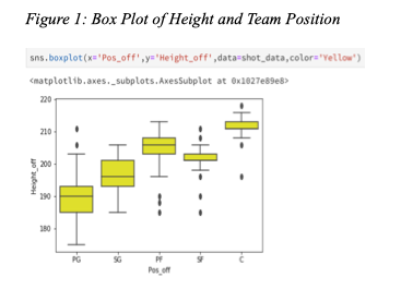
Figure 2 is a distribution plot of the shot-distance, from which a pattern can be clearly observed. Most of the shots made were concentrated to areas close to the basket or close to the three-point line (7.24 m). This makes intuitive sense because players either want to maximize probability of making the shot by being close to the basket or trying to maximize their points by trying outside the three-point line.

• The Violin Plot

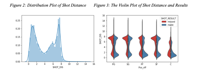
Above is the violin plot that illustrates the relationship between shot distance and shot results of different positions.

• Tableau Visualization

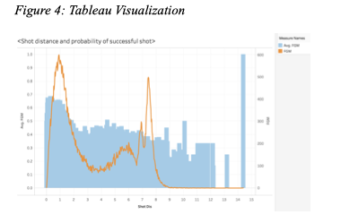
In Tableau, both the sum of field goal made and its average were plotted against the shot distance. It can be observed that number of successful shots were concentrated at the two areas discussed above. Some interesting outliers can also be observed. For example, only one shot made at a distance of 14.39 meters was successful, which was made by John Wall. Generally, the shots with the biggest success rate is when you are closest to the basket.

MODELING

In our analysis, logistics regression, decision tree and random forest model were employed because the target variable in this case is categorical, and we would like to predict whether the shot will be successful or not. Two different variable selection criteria were employed and their results will be compared. The first selection method is based on intuition, collinearity and p-value. The second one is based on feature selection method developed by William Koehrsen.

First-level variable selection

Among 45 explanatory variables in total, one who watches NBA games for a while could discover some irrelevant features when player makes a shot. For example, when considering the ability of the offender, the blocking and rebound rate of the offender seems to be of little importance on the shot results. On the other hand, the three-point shooting percentage might be insignificant to determine whether the defender could successfully hinder the shot. Therefore, we firstly deleted 23 variables that are perceived to be trivial and kept 22 independent variables in the models. Among them: 9 variables were about the offender (shooting percentage, height, etc), 9 variables were about the defender (the distance between Off and Def, rebound rate, etc), and 4 variables were about other attributes of a shot (shot clock, shot distance, etc). The details of variables are shown in the tables below.

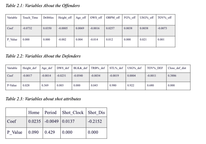
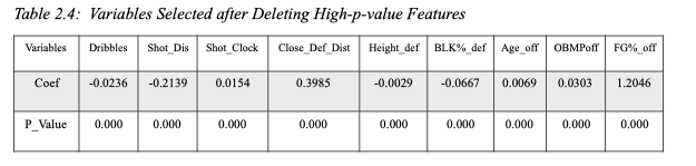
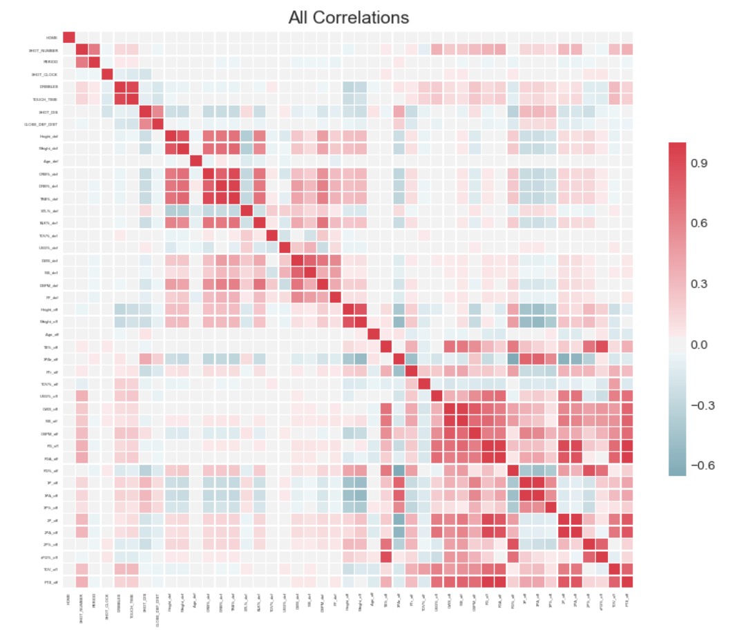
We then run the three models for the first time, but we discovered that the result for logistics regression is not optimal because some of the P-Value for certain variables were too high to be significant. Also, for decision tree and random forest, the accuracy scores were low. To further narrow down our variable selection, we plotted the heat map of both the defender variables and the offender’s variable to see which have more correlation. With the heat map, we deleted more variables and only kept the correlated ones, which are: “Dribbles”, “Shot-Dis”, “Shot-Clock”, “Close_Def_Dist”, “Height_def”, “BLK_def”, “Age_off” , “OBMP_off”, and “FG_off”

With the variables at hand, we perform the decision tree and random forest model separately with all the variables above. The results are shown before, where one could observe a significant increase in accuracy and F1-score for random forest than the decision tree. For the decision tree, we identified the importance of each variables. For random forest, we run both 100, 200, 300, and 400 and found out that 400 gives us the highest accuracy and F1 scores.

Feature Selection Model

To test whether the variables selected by intuition is on the right track, we find another model posted in Github whose goals is also to select the best-fitting features to the model, except for sklearn, another statistical package imported to this model is “LightGBM”, in which gradient boosting machine is used. The detail mechanism of this model is shown in the Jupiter Notebook files named “Feature Selector Development” and “Feature Selector Usage”.

The feature selection model developed by William is based on five selection standards:

1. Excluding the variables that have the missing fraction greater than a specified threshold.
2. Excluding variables that only have a single unique value.
3. Excluding variables that have correlation coefficient larger than a given value.
4. Excluding the variables that with 0 importance based on gradient boosting machine.
5. Excluding features that do not contribute to a specified cumulative feature importance from the gradient boosting machine.

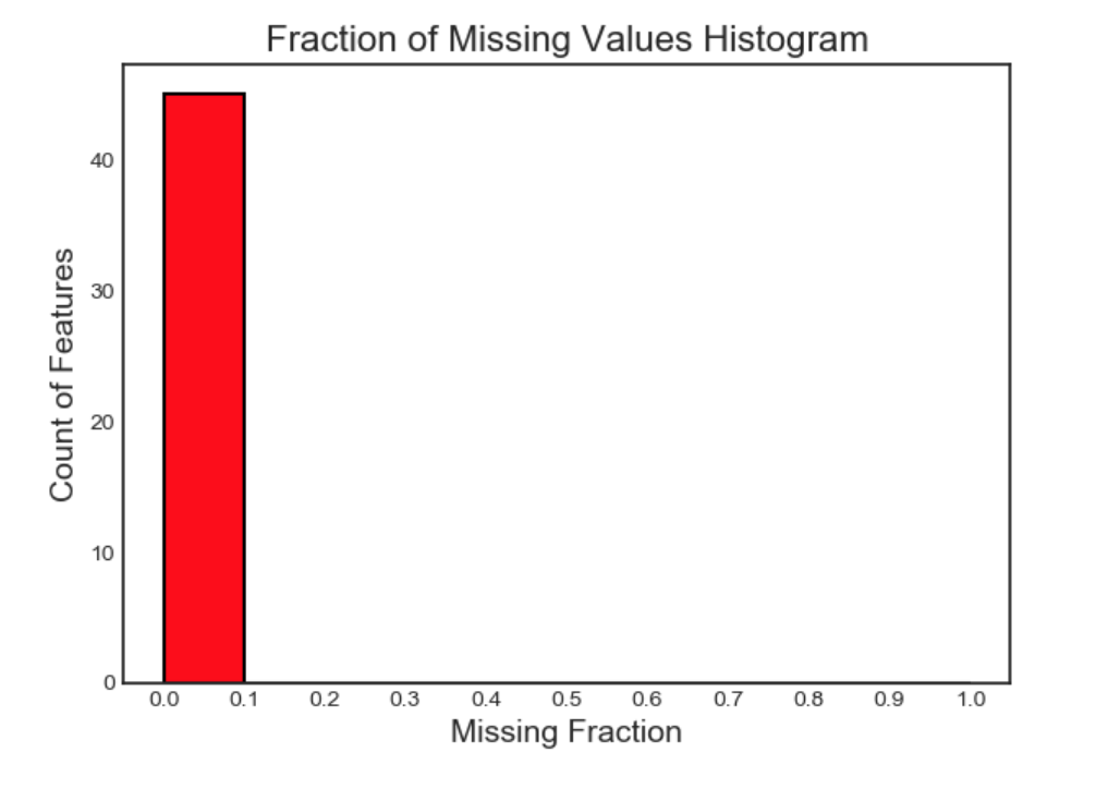
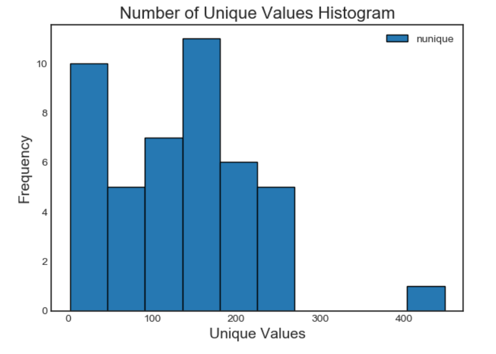
We already performed the data cleaning process by replacing the missing value with league’s average data. Also, as each shot’s attribute is quite different, we do not have variables that only have single unique value. These two features is shown in Figure 5. Thus we have 0 variable being excluded by the first and second standard.

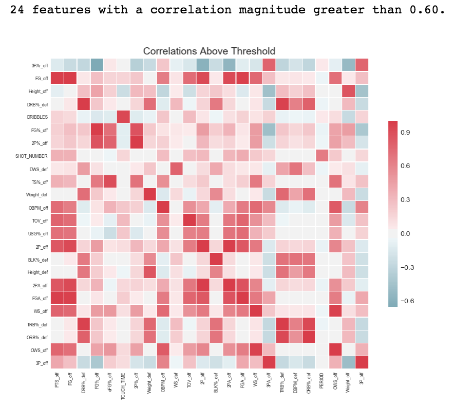
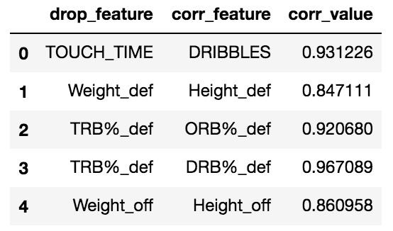
As two highly correlated variables would overshadow the effect of the other one, therefore we only need to keep one of them and deleting the others. Similar to the heat map used in the previous selection method, but William’s model provides the threshold of correlation and could exclude the variables whose correlation is above the set threshold. Here we set the correlation upper limit to be 0.6, which means we delete the features whose correlation is higher than 0.6. Figure 6 demonstrates the correlation of all variables included and those whose correlation is higher than 0.6. In this step, we delete all 24 variables (Table 3) that have the correlation above the threshold. Figure 7 is an example of the correlation value and which variable to keep or remove.

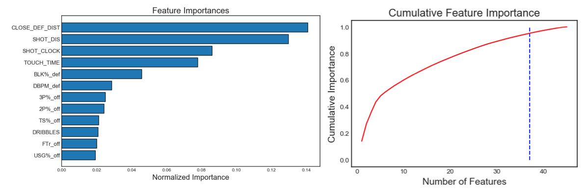
The fourth and fifth selection criteria are built on a supervised machine learning model, which remove the variables according to their estimated importance level using a gradient boosting machine in the LightGBM library. In these two steps, we remove features with zero importance and those variables that do not account for 95% of accumulative importance. The gradient boosting training process is shown below in Figure 8. After the modeling we find out that all variables are with positive importance level, and 36 variables required for 0.95 of cumulative importance. Table 4 demonstrates the 12 variables with highest importance, as well as how do those 36 variables accumulate to account for 0.95 importance. The remaining variables are ‘3P_off’, ‘PERIOD’, ‘TOV_off’, ‘Height_off’, ‘2PA_off’, ‘FGA_off’, ‘PTS_off’, ‘3PA_off’, ‘HOME’ and they are excluded — they only have relatively little contribution to predict the shot result.

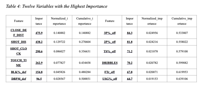
These low importance variables might have overlaps with high correlation variables, therefore the Feature Selection model totally removes 26 variables which are ‘HOME’, ‘FG_off’, ‘Height_off’, ‘DRB_def’, ‘FG_off’, ‘eFG_off’, ‘TOUCH_TIME’, ‘2P_off’, ‘Weight_def’, ‘OBPM_off’, ‘WS_def’, ‘TOV_off’, ‘2P_off’, ‘BLK_def’, ‘2PA_off’, ‘FGA_off’, ‘WS_off’, ‘3PA_off’, ‘TRB_def’, ‘DBPM_def’, ‘ORB_def’, ‘PERIOD’, ‘OWS_off’, ‘Weight_off’, and ‘3P_off’. With the remaining features, we apply logistic regression, decision tree, and random forest to further analyze whether our intuitive variable selection and modeling variable selection produce distinguished results.

Further Variable Selection

Except for variable selections based on their importance level, collinearity, and p-value as shown in previous sections. We could also use recursive feature elimination to examine whether our model include the variables that might still could be removed for improvement. Our RFE model shows that all variables’ label is “TRUE”, which means it is unnecessary to remove any of them.

rfe = RFE(model,19)
rfe = rfe.fit(X_train, y_train.ravel()
print(rfe.support_)
print(rfe.ranking)

Stepwise regression is another way to find the most suitable features to include in our model by using the backward elimination (deleting variables from full-feature model) or forward elimination (adding variables from empty model). However, owing to the word limit, our report would not include this method. If length permitted, researchers could take a look into the stepwise regression to find out whether there would be a better models containing different variables.

RESULTS & EVALUATIONS

Result from First variable selection

Our business objective is to predict as accurately as possible whether a shot will be made or not, so the accuracy of the models is important and should be ranked and compared. To compare the results and accuracy of each models, we calculated the accuracy score and F1 score of logistics regression, decision tree, and random forest models. We compared the different precision, F1 score between the three models. We found that the accuracy for logistics regression was bigger than decision tree, but it was similar to the random forest model. Logistics regression also has the largest F-1 score. Therefore, logistics regression is the most accurate model to employ in this case.

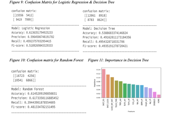
In decision tree analysis, the variable with the highest importance level is Shot Distance (0.14), the next one is Shot Clock (0.11), followed by Closest Defender Distance (0.1). It is shown that deciding variables are not the player’s own attributes. The reason may be that we used the whole NBA data to base our model on, which likely will measure an average player’s capabilities. Therefore, in the average area, player’s skills do not matter that much. What is important is the circumstances under which the offense was taken. This insight is important for coaches, and basketball players in finding the best strategy in a game and fully utilizing each person’s potential.

Feature Selection Result

We later perform logistic regression, decision tree and random forest model to the variables selected based on 5 standards from Feature Selection Model, and the results are shown as follows.

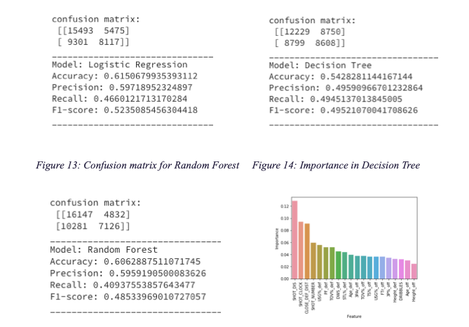
As can bee seen from the results above, the accuracy and F-1 score of logistics regression model is the highest among the three models. The results based on feature selection also are highly similar to that based variable selected by intuition and correlation.

Evaluation of Results

Six of our predicted results above show that the both decision tree models perform worse than the other two models, which could probably because our models include too many variables and thus introduce the overfitting problem. This situation, reflected by the accuracy and F1-Score, has improved in the random forest model when we set many trees to jointly predict our results. Nevertheless, the logistic regression produces the similar output confusion matrix with the random forest (a little bit higher in F1-score even). And it is easier for interpret the result in the NBA’s context. For example, if we use the average data for the 9 variables chosen in first selection method, we could predict the player’s chance of making that shot is 44.08%.

However, no matter which variable selection model we use, our best prediction results is limited to around 0.61 accuracy and 0.52. There is little difference between our intuitive variable selection model and William’s feature selection model. The possible explanation for the similarity is that, despite the difference in the number of variables included, both models include those variables with highest importance value like “SHOT_DIS” (shot distance), “CLOSE_DEF_DIST”(distance between defender and player) and so on, and those are the determined factor to the prediction.

Under both variable selection models, our prediction performance is also far from satisfaction. We believe the data constrain is one important limitation to our model. We only have one-dimensional data — distance of the shot, however the shot’s condition is measured by the three-dimensional data with location of the shot and height of the shot. Also, we try to use seasonal data to predict player’s specific game’s performance. While the player’s performance are not always constant and variability is common among all NBA players. Finally, we ignore the team-level influence which is the most important thing on the court. Basketball is never a one-on-one game, but the team cohesive, team morale, and team strategy are something hard be measured by the data.

RECOMMENDATIONS, CHALLENGES AND MITIGATIONS

Team Strategy Development

Despite having individual strengths and weaknesses, all the NBA players are highly skilled, thus making their skills not highly correlated to their success or failure. Instead of focusing on refining and improving individual skills, it is more critical to develop cohesive team strategies.

The actions that the coaches could employ would be developing these strategies using our model prior to the games, and ensure that the teams have the time to practice following these strategies. This will be value-adding for teams to increase their chances of winning. The challenge with this recommendation comes from the tradeoffs in training time that basketball players and the coaches have to sacrifice. The coach may not have the time to use the model to develop game strategies amongst many other matters that he/she will need to prioritize. These benefits of focusing on team strategies are impossible to prove, thus they may not see the need and advantages of doing so. It is also hard for players to follow a specific strategy when they are moving because it is natural to follow one’s instincts than processing information in sports. The players’ performance is also affected by a wide range of factors, making our model less accurate and effective.

To further convince these stakeholders, we can prove the validity of our model. In the future, it would be also worthy to include data from the most recent seasons and more detailed player information, such as the players’ left or right handedness and personal state into our model.

Emphasis on Team Morale

To maximize players’ performance, it is also important to ensure that everyone is in their best physical and mental being to increase their chances of outperforming their regular state. Balancing training and leisurely activities that boost team morale prior to the game is another strategy that can employed.

A key initiative that the coaches can take would be scheduling more team building or social activities prior to the game, again increasing their chances of winning. The challenge with this recommendation again lies in the tradeoffs of losing training time and the unforeseeable benefits of these tradeoffs. Another challenge is that the charm of sportsmanship lies in the possibility of creating the impossibility. If there are no miracles in sports competitions, then we will lose all the joy that we derive from chasing miracles.